Using ML to Find the Funniest Friend in FRIENDS

After finishing Andrew Ng’s machine learning courses, I decided it was time to try a project of my own. Part of what I like about ML is how it can be applied to almost anything. With that in mind, I wanted to try a project that hadn’t been done before.

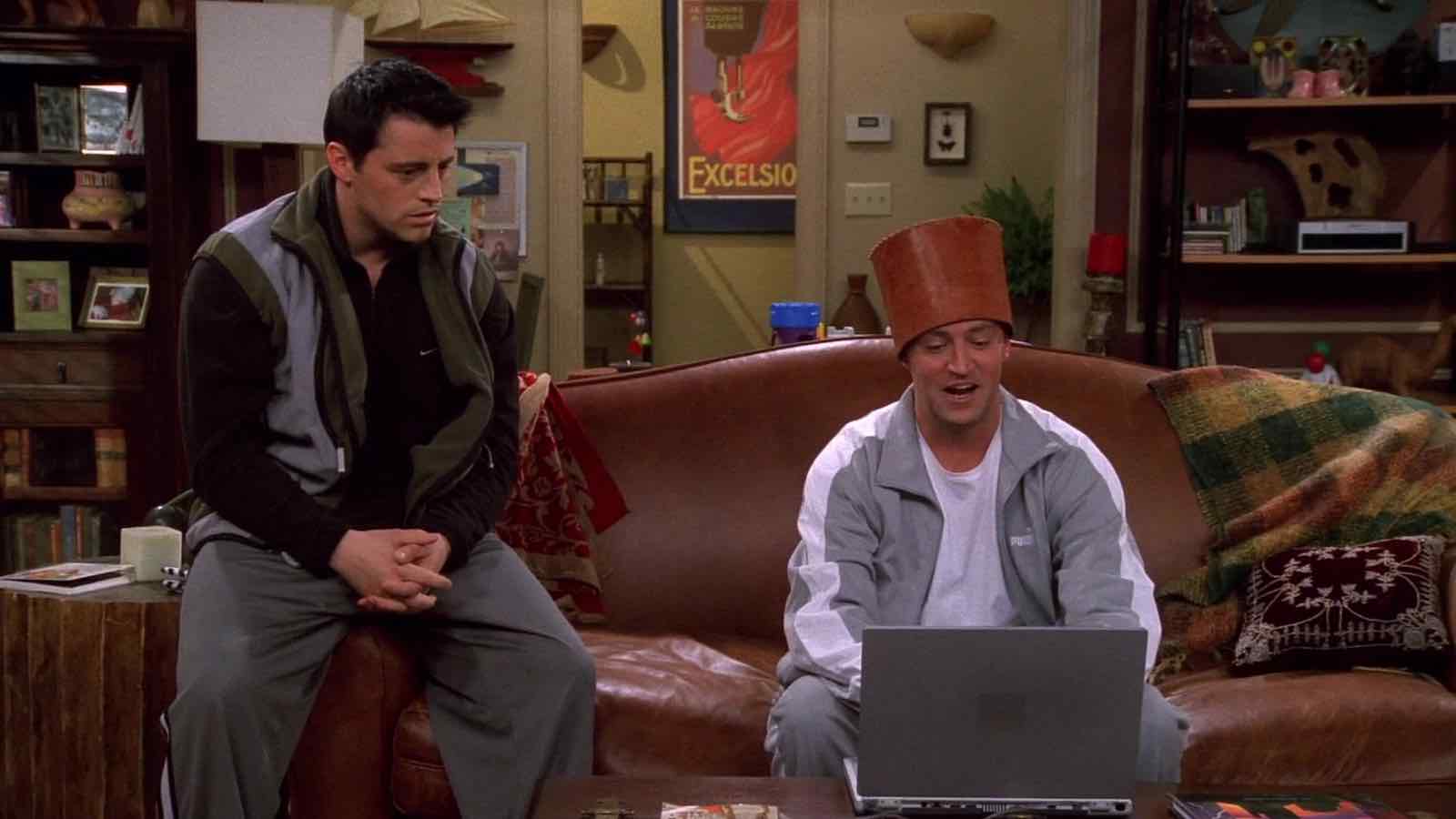
I settled on finding the funniest friend in FRIENDS because it seemed like an unanswered question and because it’s something that my non-technical friends might find interesting.

In order to find the funniest friend in FRIENDS, we need to know which character generates the most laughter (per line). There are two caveats that I explain in the results article (which you should check out if you haven’t yet). The first is that we assume audience laughter (and length of laughter) maps to how funny a spoken line is. The second caveat is that we can’t capture purely non-verbal humor, which turns out to be ~3% of the show’s laughter (this is a rough calculation based on laughter’s proximity to spoken lines).

There are three main parts to figuring out which character is responsible for which laughter. First is identifying who is speaking and when. Second is identifying laughter and when it occurs. Third is piecing together the first two parts to figure out who is responsible for each instance of laughter.

Part 1

The Who and the When

I talked the project over with some friends who know more about ML than I do. They advised me that the first part of the project (who is speaking when) is non-trivial when it comes to voice recognition algorithms. Detecting and differentiating human voices is still a difficult problem for ML. I read some papers and articles and it seemed to confirm my friends’ sentiments. Here is an example of an article that can identify different human voices with 80-85% accuracy. For my project, I didn’t think 80-85% accuracy would be high enough to draw any sort of conclusions about the funniest friend. That said, if you know of a relevant model for this sort of task please reach out!

With voice recognition ML not likely to perform accurately enough, I decided to try some different approaches. Because FRIENDS is so popular, there are fan-created script files for every episode in the show. These script files tell you who is speaking and what they say:

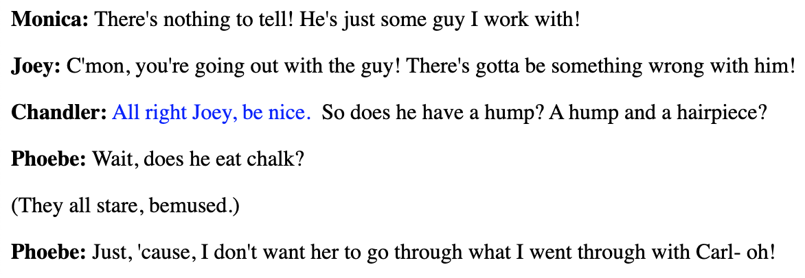
There have even been some data science articles written that make use of this script dataset in order to find interesting facts like who had the most speaking lines across all 10 seasons of the show.

These script files are great but they don’t tell us exactly WHEN any of these lines are said during the episode. Luckily, there are also subtitles files for each episode of the show. They tell you what is said and when it is said, but not WHO said it:

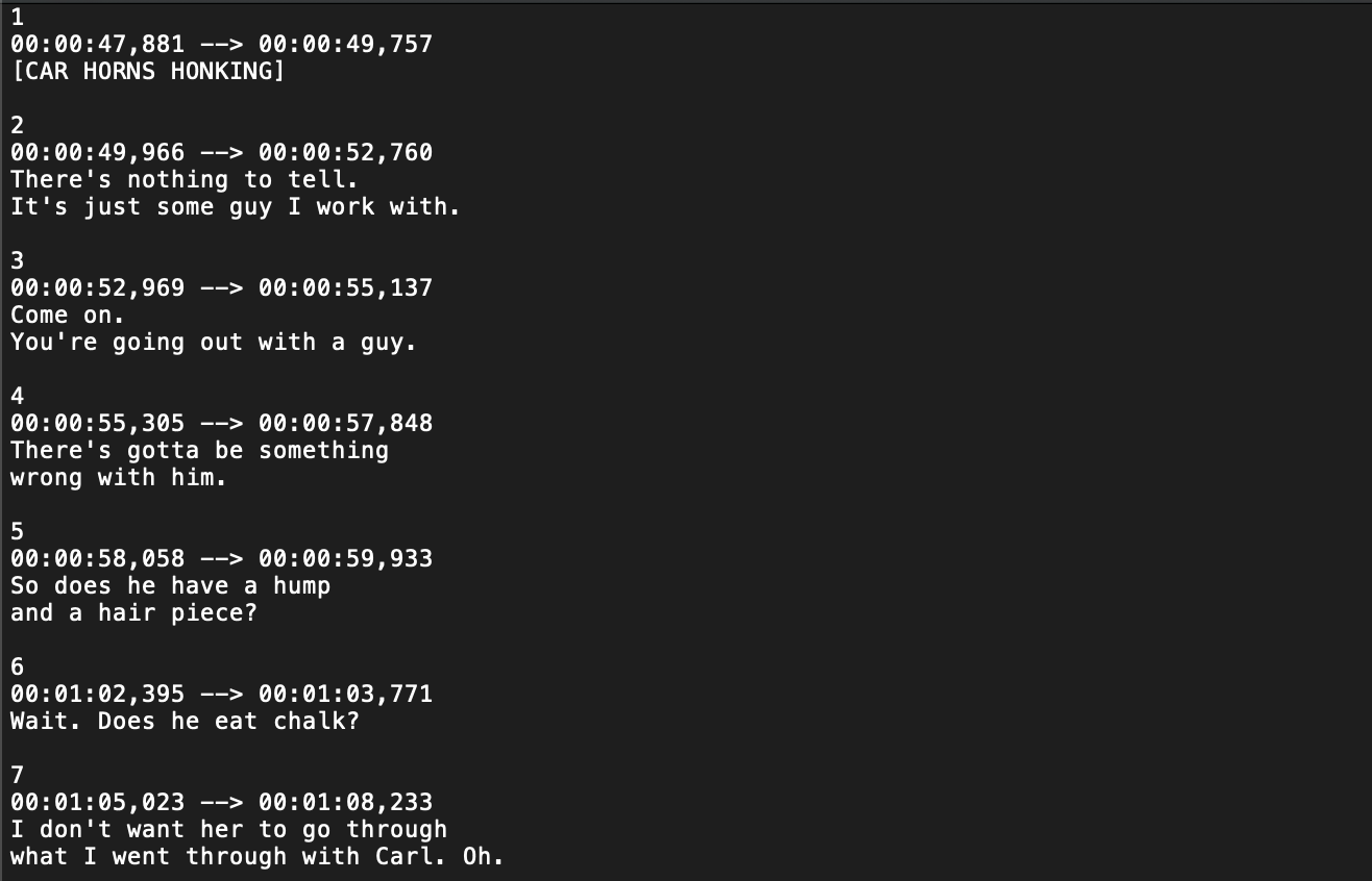
If we could somehow combine the script file and subtitles file, we could get the WHO and the WHEN that we need in order to figure out who speaks right before laughter. The script and subtitles both contain the WHAT (the spoken lines) so we can join them together using the WHAT to map the WHO to the WHEN.

If you look closely at the script and subtitles images above, you can see that mapping the lines to each other won’t be as easy as it sounds.

Quick note: There is a lot of code in this project so I don’t post much of it in this article. Instead I will point you to the relevant Jupyter notebook on Github if you’re interested in following along with the implementations. If you’re interested in the scraping of script and subtitles files, see this notebook.

I ended up using a series of 3 algorithms to join the script and subtitles files of each episode based on their spoken line similarities. Find the implementations here.

Algorithm #1

One character word/phrase match

We look for unique words or unique phrases (up to 5) in the script that are spoken by only one character and we see if that unique word or phrase also appears in the subtitles file (an equal or lesser amount of times). We then assign that character to the lines containing the unique word or phrase in the subtitles. An example from Season 1 Episode 1 is that Ross is the only character to say “should I know” in the episode, and these three words appear together once in the script and once in the subtitles. Therefore we assign the unknown subtitles line containing “should I know” to Ross.

We get about 80% of all the lines in the subtitles after algorithm #1 and those lines were also about 99% accurate in terms of getting the character right.

Algorithm #2

Local one character phrase match

This algorithm is the same as Algorithm #1 except that it is applied to specific parts of the script and subtitles files. The idea is that we can now start to zoom in on areas of the script where we have unknown lines between two known lines. We can do a one-character “unique word or phrase” match in that smaller area and find matches we would not have found if we were looking across the entire episode. We know exactly which line we are looking for in the subtitles and we also know where the closest known line above and below that line is in the subtitles.

However, we don’t have our bearings in the script file at all. To get our bearings, we take the “unique word or phrase” that gives us the known line above in the subtitles and same for the known line below. We then search the script file for a pattern that looks something like “known-line-above word”, then unknown line, then “known-line-below word.” Because known lines can have the same discovery word (for example, 4 different lines in the subtitles file for S1E1 have the discovery word “daddy”), this process is not flawless. But once we choose a “range” of the script to search, we simply execute algorithm #1 locally in that range.

To explain how this algorithm is different from algorithm #1, imagine the phrase “How are you?” is said 5 times throughout an episode by 3 different characters. Algorithm #1 would not be able to match any characters in this situation. But if we already know lines 45 and 55 we can search between these two lines. We find that “How are you?” is said only once by one character. Now we can match that character to a line where we couldn’t before.

After Algorithm #2 we end up with 93% of lines predicted and 98% accuracy on those predictions. Algorithm #2 contributes an extra 13% with ~92% accuracy. Not as accurate as Algorithm #1, but not terrible either.

Algorithm #3

Exact Speaker Count

Now say we know lines 45 and 48 in the script. Obviously there are 2 lines in between 45 and 48. The corresponding subtitles line numbers will be different and there may even be a different number of lines in between. But if there are 2 lines in between in the subtitles and script, we can simply map the two characters in the script to those two lines in the subtitles in sequential order. This situation is more rare than you’d think so Algorithm #3 only adds another 2% of total lines.

After Algorithm #3, we now know 95% of lines with 98% accuracy.

With 98% accuracy on 95% of lines, I presume we are outperforming what a voice recognition ML model could get us (again, if you know of a super accurate model, please reach out!). The last 5% of lines tend to be extremely difficult to label. For example, Rachel will walk into a room of 3 friends and they will all say “Hi” to each other, nearly simultaneously. Without using a beastly combination of voice recognition, on-screen character (image) recognition, and text processing with the subtitles and script files I believe it would be very difficult for a model or algorithm to label these lines accurately. Therefore, I simply hand-labeled the last 5% of lines (hopefully with near 100% accuracy). This means that overall, the first part of the project will have character lines that are labeled with ~98% accuracy.

From here, I do a quick check of all unique names across the 10 seasons and I assign any aliases to the correct characters. Then upload the labeled data into a SQLite database.

Part 2

Recognizing and Labeling Laughter (Actual ML Involved!)

For recognizing laughter, there is no text-based file that I’m aware of that could give us the data we need. So we must go to the actual audio.

I started with the video files of each episode for all 10 seasons. From there we can use VLC (on Mac) to convert video files to audio (MP3).

Once we have the audio files, there is a transform we can apply that I found helps the ML algorithm tremendously.

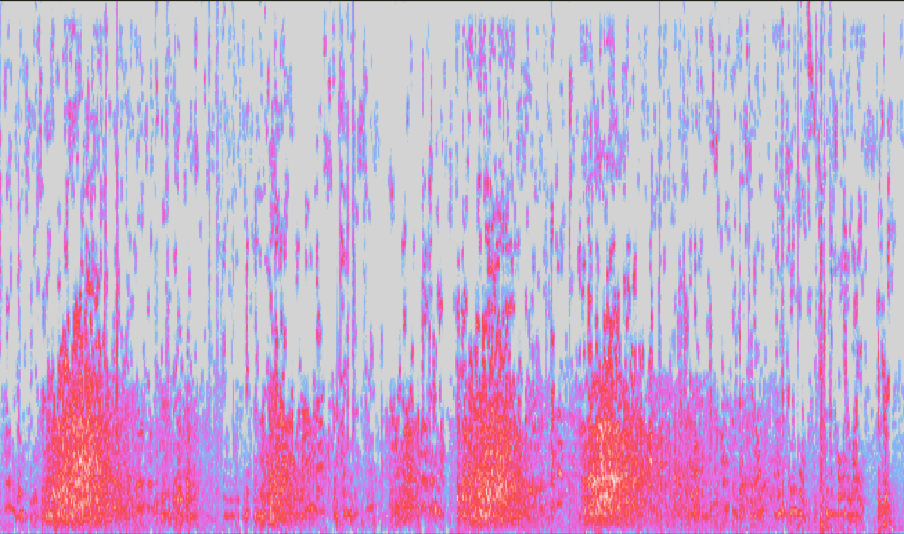
We take the stereo MP3 track and split it into a dual-channel mono track, then invert one of the channels which effectively cancels out anything that was center-panned in the original stereo track. This is usually the character vocals. I use a free software called Audacity to accomplish this. This gives us an audio track that effectively silences the characters’ speech and leaves nearly all of the audience laughter alone. Here is the method.

I will note that this method doesn’t work anywhere near perfectly (a lot of vocals come through still) but it can make a tremendous difference for helping the ML algorithm recognize laughter. Take a look at a 25-second clip before and after this transform. Hint: The yellow areas of the second clip are true laughter.

Before:

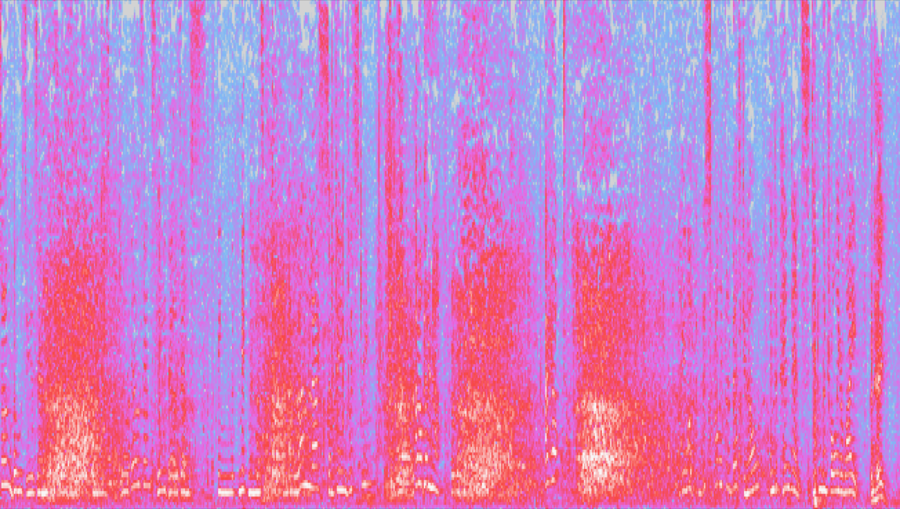
After:

Now we have the base audio that we will feed to our ML model.

In order for the model to learn, we need to give it the “answers” for a few episodes. In order to get training examples, I went through 20 full episodes in Audacity and labeled the laughter examples. You can easily export the labels as text files.

While I was taking Andrew Ng’s Deep Learning course on Coursera, there was a very relevant project on detecting trigger words (like “Hey Siri”) from audio clips. The ML model used a 1-D convolutional layer and 2 GRU layers. I thought this model would be a good starting point.

For ease of use, I cut the 22-minute episodes into 10-second clips.

For the model to “understand”, we have to translate our audio into numerical data. We can represent the audio clip to the model as a number of time steps (splitting the 10-second clip into roughly 10-millisecond increments) and display the values of different audio frequencies at each time step. I ended up with 257 frequencies per time step and 861 time steps per 10-second clip. So a 10-second clip becomes a numpy array with shape (861, 257). You can find the audio data preprocessing notebook here.

The model also needs “answers” to train on. To generate the y input, we use those text files full of hand-labeled laughter ranges. At each timestep of each 10-second clip, we basically ask the question, “Is this timestep inside a laughter range or outside?” and we label it “1” if it is inside a laughter instance, and “0” if not. For a 10-second clip, the y value will be of shape (861, 1) because we simply have a binary output at each time step in the clip.

Side note: I ended up doing everything in Part 2 using Kaggle notebooks. I ran into disk space and RAM issues so many times that I wouldn’t recommend it for a project of this size. I understand Google Colab notebooks suffer similar restrictions. The appeal of these options is that you get free GPU time (30 hours per week) and unlimited access to 16 CPU cores. In the future, I would likely look towards a paid computing option to save myself the memory headaches. It turned out utilizing a GPU on a Kaggle notebook only had about a 15% improvement in training time. So for this project, a GPU may not have even been necessary. Here’s the notebook where I train the model.

We grab the X and y datasets and split them into 60% train, 20% development and 20% test.

From there we define our model beginning with a 1-D convolutional layer and 2 GRU layers followed by a dense layer. I experimented with more or less GRU layers and also different combinations of dropout and batch normalization layers but this combination seemed to work best. It happened to be the exact same combination Andrew Ng’s “trigger word” model used. Maybe he knows what he’s talking about after all.

We use the Adam algorithm for gradient descent optimization as well as a binary cross-entropy loss function.

Finally we can train the model!

When I was experimenting with different hyper parameters and layer combinations I found that using 15 epochs was more than enough to figure out if the model would perform better or worse than past models. This took between 15-30 mins for most combinations. For the final model I decided to use, I trained for 100 epochs which took about 3.5 hours on a GPU.

The best model was able to identify laughter with 95% accuracy. I tried to do better than 95% for a long time. But what I eventually figured out was that a lot of the error was my own fault (i.e. human error). I didn’t realize this until I went back and labeled the laughter for an episode that I had already labeled a week prior. I then compared the labels and found that they only had 97% overlap! Meaning that the “human” level accuracy for identifying laughter in this situation is ~97%, so it is unreasonable to expect a machine to do better than 97%. In that light, 95% for the algorithm looks like a more positive outcome.

Even with 95% accuracy, the model almost never misses a laughter instance. The 5% error tends to come from the very beginning or end of a laughter instance where it is often less clear when laughter “officially” begins or ends.

Once we have the trained model, I use it to predict laughter for all the non-labeled episodes. I did this outside of the Kaggle environment because of the massive amount of data we are predicting (all 10 seasons of audio effectively). Notebook found here.

With the predictions in hand, there are two post-processing steps I take in order to make the laughter ranges more sensible. Anything under 400ms is too short to be a standalone laughter instance, so I decided it either needs to join together with a close-by laughter instance, or it needs to be removed. Any gap of 100ms or less between two laughter instances is much too short to be meaningful, so we combine those two laughter instances into one longer laughter instance.

We take our processed predictions and store them in SQLite where they are now ready to be combined with the character data from Part 1.

Part 3

Part 3 notebook found here.

We bring in both datasets and format them to be compatible with each other.

Then we use a simple minimization function to decide who caused each instance of laughter. We take the beginning timestamp of the laughter instance and we find the minimum distance to the end of a character line. Whichever character’s line ends closest to the beginning of the laughter (within +/- 3 seconds) is the character to whom we attribute the laughter instance.

Now we have the exact data we need to answer “Who is the Funniest Friend in FRIENDS?”

But first, to make sure everything is working correctly, I create custom subtitles for each episode that will show us the output in real time.

SRT files (subtitles files) are just text files with a standardized format for displaying subtitles on a video. We convert our timestamps and speaking lines into SRT format and we can combine it with any video file. Here’s the demo:

Once we can see that the labels are working well in practice, all that’s left is to calculate the answer to our original question.

Like I mention in the results article, it would be unfair to simply add up the seconds of laughter for each character across all 10 seasons to see who is funniest. That’s because some characters have many more lines than others. So I believe a more fair way to calculate the funniest character would be to see how much laughter follows each line spoken by a character on average. The character with the most seconds of laughter following each of their lines on average, wins.

A couple SQL queries later, we can see that it turns out to be Joey with 1.27 seconds of laughter per line on average! But wait there’s more…

How accurate are these findings?

It’s easy to look at a chart with precise numbers and “trust” that the data is accurate. But we all know this isn’t how the world works. So what are the chances that Joey ISN’T the funniest character?

We know Part 1 predicted the correct character for subtitle lines ~98% of the time (I painstakingly hand-labeled ~1000 lines to test it). And we know for Part 2, our ML model was ~95% accurate in labeling each ~10ms timestep of laughter correctly. For Part 3, deciding who is responsible for each laugh, I did more manual testing on a few episodes (~300 examples) and found that we attribute laughter to the correct character about 95% of the time. But our final metric, Joey’s 1.27 seconds of laughter per line, is a bit more complicated. It combines getting the character correct (~95%) and getting the length of laughter correct (~95%). On a timestep by timestep basis, the probability of both events being correct is ~90% (95% * 95%).

With this in mind, we can calculate confidence intervals around Joey’s 1.27 seconds of laughter per line. A 95% confidence interval gives us a +/- 0.02 seconds range around Joey’s 1.27 average seconds of laughter. In second place, Chandler’s 1.22 seconds of laughter also has a 95% confidence interval of +/- 0.02 seconds. This means we have greater than 95% confidence that Joey is the funniest character because Chandler’s best case value of 1.24 can’t surpass Joey’s worst case value of 1.25 within our 95% interval!

On the other hand, Chandler and Phoebe’s intervals DO overlap which means we can’t be confident about the 2nd funniest character. And we also can’t be sure about the least funny character because Rachel and Monica’s intervals overlap as well!

I hope you enjoyed this walkthrough. If you’re working on a similar project, feel free to hit me up. Or if you have questions about any methods in this article or in my notebooks, please reach out as well. I would especially enjoy suggestions on improvements to this project! You can find my contact here.